Back to Main Menu

Degradation Profiles

The Degradation Profile is the foundation of Strategic Asset Life Cycle modelling.

Assets typically start off as brand new (service state 0), and at some future point in time, the asset will have transitioned to end of life (service state 6).

 

To model this process we therefore define life cycle degradation profiles, simulating an asset's degradation (the way it moves from one service state to another throughout its life cycle). This is one of the most important steps in Brightly Predictor. The life cycle degradation profiles configured in Predictor describe the relationship between useful life, remaining life, service potential and native scaling (which are all assigned to a Service State) of an asset.

 

The following explains the relationship between service state, remaining life, service potential and native scale, which are all integral to configuring life cycle degradation profiles.

Service State is a numerical integer value between 0 to 6, which reflects the measure of the condition, performance, physical integrity, health or similar measure of an asset or asset component consistent with the International Infrastructure Management Manual (IIMM) and ISO 55000 guidelines. The life cycle degradation profile describes the relationship between useful life and remaining useful life (assigned to each Service State) of an asset. In essence, the Service State reflects where an asset or asset component is within its defined useful life at any given point in time.

 

Service Potential is defined in the IIMM as “The total future service capacity of an asset. It is normally determined by reference to the operating capacity and economic life of an asset”. In simple terms, the Service Potential expresses the available service level that the asset or asset component will provide.

 

Whilst Service State reflects where an asset or asset component is within its defined useful life at any given point in time, the corresponding Service Potential reflects the remaining available service level. In the absence of historical and/or existing Service Potential performance data, generally to begin with and when configuring the degradation profile, ‘Service Potential %’ is aligned to reflect the ‘Remaining Life %’ and hence the values are the same.

 

Native Scale offers organizations the ability to define and align the Service State values using a scale that is ‘native’ to the organization. For example, ASTM D 6433-03 (commonly used in North America) defines the pavement condition index (PCI) as a numerical rating between 0 to 100 where 0 is the worst possible condition and 100 as the best possible condition. Another example is the International Roughness Index which is represented as a number ranged between 10 to 1 that reflects the roads overall ride quality, where 1 is the best possible condition and 10 the worst possible condition. Both Native Scales can be configured in Predictor using separate life cycle degradation profiles.

 

This feature provides users with the ability to define the relationship between values that are ‘native’ to the organization with the asset or asset component’s remaining useful life.
The relationship between Service State, Service Potential, and Native Scale is defined by the user in the life cycle degradation profile section of the Template. In defining this relationship, 0% Service Potential is always equal to a Service State of 6, and a Service Potential of 100% is always equal to a Service State of 0. Native Scale must always have a maximum value and a minimum value, but the scale can be defined in either descending or ascending order, between any two whole number values.

 

An asset's exact life cycle degradation profile is influenced by a range of factors which can include the assets or asset components current condition/performance, design, age, environmental factors, usage and user behavioural patterns, quality of raw materials and construction practices.
Different degradation profiles specific to each asset or asset component type can be configured within the Template, and as a model matures additional degradation profiles can be added to improve accuracy.

 

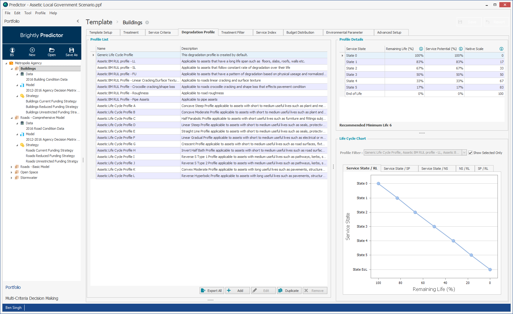
Predictor contains 12 pre-configured fixed degradation profiles which can be used to model the Life Cycle degradation profile of an asset, and also allows for users to add and configure their own degradation profiles.

 

Individual degradation profiles can be exported by right-clicking and selecting 'export', or the full list can be exported with the 'Export All' button.

 

Degradation Profiles can be copied using the ‘Duplicate’ button and then modified using the ‘Edit’ button, and new degradation profiles are added using the ‘Add’ button:

 

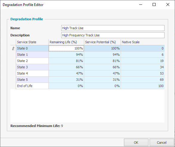
The Remaining Life percentage and Service Potential percentage values are configurable for each condition state by clicking in the appropriate cell and inputting a value, which must be less than the previous state. Remaining Life is expressed as a percentage value between 0% and 100% where 0% indicates no life available and 100% represents full life available.

 

Service Potential is also expressed as a percentage value between 0% and 100%, where 0% indicates no Service Potential and 100% represents full Service Potential available.

 

Native Scale must always have a maximum value and a minimum value and must be between any two whole number values. However, the scale can be defined in either descending or ascending order.
Some examples of user-defined Native Scale ranges are as follows:

• 0-100
• 100-0
• 1-10
• 10-1
• 0-500

 

The default native scale values in the pre-configured fixed degradation profiles reflects the 0-100 range and are calculated for each service state using the following equation; 100-Service Potential%.

 

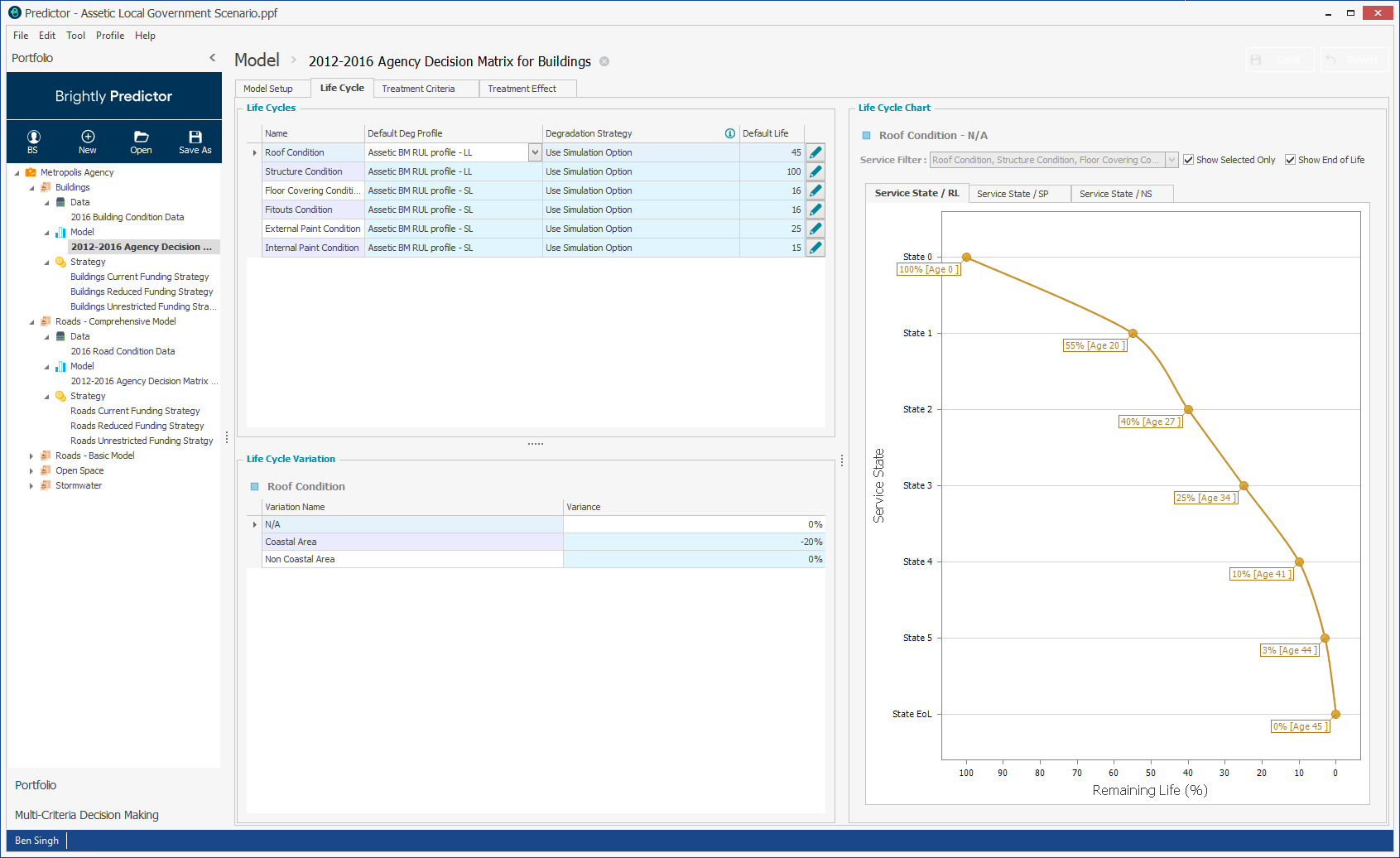
To set a Life Cycle:

• Click the Life Cycle tab
• Select the Degradation profile to use in the drop-down in the life cycles box: